

概要
加速度センサーシリーズの続編です。
前回までは、正常か異常かを判定する仕組みを作りました。
しかし実際の設備保全では、異常と分かっただけでは十分ではありません。
保全担当者が本当に知りたいのは、「何が起きているのか」です。
そこで今回は、PCAとSVMを使って、振動データの特徴から異常の自動判定に挑戦してみました。
詳しくは、以下のYouTube動画をご覧ください。
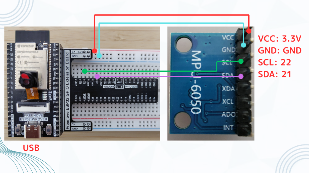
配線
プログラムコード
マイコン(ESP32)
・MPU6050で、X・Y・Z方向の加速度を計測
・合成加速度 acc_total を計算
・1000Hz周期でデータ取得
・CSV形式でシリアル出力
#include <Wire.h>
#include <MPU6050_tockn.h>

MPU6050 mpu(Wire);

const unsigned long SAMPLE_US = 1000; // 1000us = 1000Hz
unsigned long last_us = 0;

void setup() {
  Serial.begin(115200);
  Wire.begin(21, 22);
  Wire.setClock(400000);

  mpu.begin();
  mpu.calcGyroOffsets(true);

  Serial.println("time_us,ax,ay,az,acc_total");
}

void loop() {
  unsigned long now = micros();
  if (now - last_us < SAMPLE_US) return;
  last_us = now;

  mpu.update();

  float ax = mpu.getAccX();
  float ay = mpu.getAccY();
  float az = mpu.getAccZ();
  float acc_total = sqrt(ax*ax + ay*ay + az*az);

  Serial.print(now);
  Serial.print(",");
  Serial.print(ax, 4);
  Serial.print(",");
  Serial.print(ay, 4);
  Serial.print(",");
  Serial.print(az, 4);
  Serial.print(",");
  Serial.println(acc_total, 4);
}
Python
正常モード、故障モードA、故障モードBの3種類のデータをあらかじめ用意し、検証用のデータがどれに分類されるか確かめるためのコードです。
import os
import glob
import numpy as np
import pandas as pd
import matplotlib.pyplot as plt

from scipy.interpolate import interp1d
from scipy.signal import welch, find_peaks, peak_widths
from sklearn.preprocessing import StandardScaler
from sklearn.decomposition import PCA
from sklearn.svm import SVC


# =========================================================
# ① ここだけ設定すればOK
# =========================================================

BASE_CLASS_DIR = r"C:\Users\**************************************************"
# ↑ normal / ModeA / ModeB / validation フォルダを置いている場所に変更してください

TRAIN_DATA_DIRS = {
    "normal": os.path.join(BASE_CLASS_DIR, "normal"),
    "ModeA":  os.path.join(BASE_CLASS_DIR, "ModeA"),
    "ModeB":  os.path.join(BASE_CLASS_DIR, "ModeB"),
}

VALIDATION_DIR = os.path.join(BASE_CLASS_DIR, "validation")

FILE_PATTERN = "*.csv"

FS = 1000.0
# 第2回で1000Hz測定した前提です

CHANNEL = "acc_total"
# 3軸合成加速度を使って特徴量を作ります

N_PER_SEG = 1024
N_OVERLAP = 512

F_MIN = 5.0
F_MAX = 500.0
# 解析する周波数範囲です

BANDS = [
    ("band_psd_sum_5_10", 5.0, 10.0),
    ("band_psd_sum_10_30", 10.0, 30.0),
    ("band_psd_sum_30_80", 30.0, 80.0),
    ("band_psd_sum_80_200", 80.0, 200.0),
    ("band_psd_sum_200_400", 200.0, 400.0),
    ("band_psd_sum_400_500", 400.0, 500.0),
]

CLASS_COLORS = {
    "normal": "blue",
    "ModeA": "red",
    "ModeB": "green",
    "ModeC": "orange",
}

CLASS_DISPLAY_NAMES = {
    "normal": "Normal",
    "ModeA": "Abnormal A",
    "ModeB": "Abnormal B",
    "ModeC": "Abnormal C",
}

OUTPUT_RESULT_CSV = os.path.join(BASE_CLASS_DIR, "validation_result.csv")


# =========================================================
# ② CSV読み込み・等間隔化
# =========================================================

def load_and_resample_csv(csv_path, channel=CHANNEL, fs=FS):
    """
    CSVを読み込み、time_usを使って等間隔データに補正します。
    ESP32の測定データは完全な等間隔ではないため、
    FFT前に時間軸をそろえます。
    """

    df = pd.read_csv(csv_path)

    required_cols = ["time_us", channel]
    for c in required_cols:
        if c not in df.columns:
            raise ValueError(f"{csv_path} に必要列 '{c}' がありません。")

    t = df["time_us"].to_numpy(dtype=float) * 1e-6
    x = df[channel].to_numpy(dtype=float)

    mask = np.isfinite(t) & np.isfinite(x)
    t = t[mask]
    x = x[mask]

    if len(t) < 10:
        raise ValueError(f"{csv_path} の有効データが少なすぎます。")

    idx = np.argsort(t)
    t = t[idx]
    x = x[idx]

    uniq_mask = np.diff(t, prepend=t[0] - 1.0) > 0
    t = t[uniq_mask]
    x = x[uniq_mask]

    if len(t) < 10:
        raise ValueError(f"{csv_path} は重複除去後の有効データが少なすぎます。")

    dt = 1.0 / fs
    t_uniform = np.arange(t[0], t[-1], dt)

    if len(t_uniform) < 256:
        raise ValueError(f"{csv_path} は解析に必要な長さが不足しています。")

    f_interp = interp1d(
        t,
        x,
        kind="linear",
        fill_value="extrapolate"
    )

    x_uniform = f_interp(t_uniform)

    # 平均値を引いてDC成分を除去します
    x_uniform = x_uniform - np.mean(x_uniform)

    return t_uniform, x_uniform


# =========================================================
# ③ FFT特徴量を抽出
# =========================================================

def calc_psd_features(x, fs=FS):
    """
    Welch法でPSDを計算し、故障モード分類に使う特徴量を作ります。
    """

    f, pxx = welch(
        x,
        fs=fs,
        window="hann",
        nperseg=min(N_PER_SEG, len(x)),
        noverlap=min(N_OVERLAP, max(0, len(x) // 2 - 1)),
        detrend="constant",
        scaling="density"
    )

    band_mask = (f >= F_MIN) & (f <= F_MAX)
    f_sel = f[band_mask]
    p_sel = pxx[band_mask]

    if len(f_sel) < 10:
        raise ValueError("有効な周波数点が不足しています。")

    features = {}

    # 支配周波数とその強さ
    dom_idx = np.argmax(p_sel)
    dom_freq_hz = f_sel[dom_idx]
    dom_psd = p_sel[dom_idx]

    features["dom_freq_hz"] = dom_freq_hz
    features["dom_psd"] = dom_psd

    # 支配ピークの幅
    peaks, _ = find_peaks(p_sel)

    if len(peaks) > 0:
        peak_idx = peaks[np.argmin(np.abs(peaks - dom_idx))]
        widths, _, _, _ = peak_widths(p_sel, [peak_idx], rel_height=0.5)
        dfreq = f_sel[1] - f_sel[0] if len(f_sel) > 1 else 1.0
        peak_width_hz = widths[0] * dfreq
    else:
        peak_width_hz = np.nan

    features["peak_width_hz"] = peak_width_hz

    # ピークの鋭さ
    bg = np.median(p_sel)
    features["peak_sharpness"] = dom_psd / (bg + 1e-12)

    # 5Hz以上の全体エネルギー
    features["psd_sum_ge5"] = np.sum(p_sel)

    # 周波数帯ごとのエネルギー
    for name, fl, fh in BANDS:
        m = (f >= fl) & (f < fh)
        features[name] = np.sum(pxx[m])

    # スペクトル重心
    features["spec_centroid_hz_ge5"] = np.sum(f_sel * p_sel) / (np.sum(p_sel) + 1e-12)

    # 高周波比
    low_5_80 = np.sum(pxx[(f >= 5) & (f < 80)])
    high_80_500 = np.sum(pxx[(f >= 80) & (f <= 500)])
    features["hi_lo_ratio_ge80_over_5to80"] = high_80_500 / (low_5_80 + 1e-12)

    low_5_200 = np.sum(pxx[(f >= 5) & (f < 200)])
    high_200_500 = np.sum(pxx[(f >= 200) & (f <= 500)])
    features["hi_lo_ratio_200_500_over_5_200"] = high_200_500 / (low_5_200 + 1e-12)

    return features


def extract_features_from_file(csv_path):
    _, x = load_and_resample_csv(csv_path, channel=CHANNEL, fs=FS)
    features = calc_psd_features(x, fs=FS)
    return features


# =========================================================
# ④ 学習用・検証用データを読み込む
# =========================================================

def build_feature_table_for_training(data_dirs, file_pattern="*.csv"):
    rows = []

    for class_name, folder in data_dirs.items():
        paths = sorted(glob.glob(os.path.join(folder, file_pattern)))

        if len(paths) == 0:
            print(f"[WARNING] {class_name}: ファイルが見つかりません -> {folder}")
            continue

        for path in paths:
            try:
                feat = extract_features_from_file(path)
                feat["label"] = class_name
                feat["file_name"] = os.path.basename(path)
                feat["source"] = "train"
                rows.append(feat)

            except Exception as e:
                print(f"[SKIP] {path}")
                print(f"       reason: {e}")

    if len(rows) == 0:
        raise RuntimeError("学習用CSVが1件も読み込めませんでした。")

    return pd.DataFrame(rows)


def build_feature_table_for_validation(validation_dir, file_pattern="*.csv"):
    rows = []

    paths = sorted(glob.glob(os.path.join(validation_dir, file_pattern)))

    if len(paths) == 0:
        raise RuntimeError(f"validation フォルダにCSVが見つかりませんでした。 -> {validation_dir}")

    for path in paths:
        try:
            feat = extract_features_from_file(path)
            feat["file_name"] = os.path.basename(path)
            feat["source"] = "validation"
            rows.append(feat)

        except Exception as e:
            print(f"[SKIP] {path}")
            print(f"       reason: {e}")

    if len(rows) == 0:
        raise RuntimeError("検証用CSVが1件も読み込めませんでした。")

    return pd.DataFrame(rows)


# =========================================================
# ⑤ PCA + SVM
# =========================================================

def prepare_training_matrix(df_train):
    meta_cols = ["label", "file_name", "source"]

    feature_cols = [c for c in df_train.columns if c not in meta_cols]

    X = df_train[feature_cols].copy()

    X = X.replace([np.inf, -np.inf], np.nan)
    X = X.fillna(X.median(numeric_only=True))

    return X, feature_cols


def train_pca_svm(df_train):
    X_train, feature_cols = prepare_training_matrix(df_train)

    y_train = df_train["label"].to_numpy()

    # 特徴量は単位や桁が異なるため標準化します
    scaler = StandardScaler()
    X_train_scaled = scaler.fit_transform(X_train)

    # PCAで2次元に圧縮します
    # 動画ではこの2次元マップを使うと説明しやすいです
    pca = PCA(n_components=2, random_state=42)
    X_train_pca = pca.fit_transform(X_train_scaled)

    # PCA空間上でSVMを学習します
    clf = SVC(kernel="rbf", C=3.0, gamma="scale")
    clf.fit(X_train_pca, y_train)

    df_train_plot = df_train[["label", "file_name", "source"]].copy()
    df_train_plot["PC1"] = X_train_pca[:, 0]
    df_train_plot["PC2"] = X_train_pca[:, 1]

    return df_train_plot, scaler, pca, clf, feature_cols


def transform_validation(df_val, scaler, pca, feature_cols):
    X_val = df_val[feature_cols].copy()

    X_val = X_val.replace([np.inf, -np.inf], np.nan)
    X_val = X_val.fillna(X_val.median(numeric_only=True))

    X_val_scaled = scaler.transform(X_val)
    X_val_pca = pca.transform(X_val_scaled)

    df_val_plot = df_val[["file_name", "source"]].copy()
    df_val_plot["PC1"] = X_val_pca[:, 0]
    df_val_plot["PC2"] = X_val_pca[:, 1]

    return df_val_plot, X_val_pca


def classify_validation(df_val_plot, X_val_pca, clf):
    pred = clf.predict(X_val_pca)

    df_result = df_val_plot.copy()
    df_result["pred_label"] = pred

    try:
        scores = clf.decision_function(X_val_pca)

        if scores.ndim == 1:
            df_result["decision_score"] = scores
        else:
            df_result["decision_score_max"] = np.max(scores, axis=1)

    except Exception:
        pass

    return df_result


# =========================================================
# ⑥ 可視化
# =========================================================

def plot_pca_map(df_train_plot):
    plt.figure(figsize=(10, 8))

    for cls in df_train_plot["label"].unique():
        sub = df_train_plot[df_train_plot["label"] == cls]

        color = CLASS_COLORS.get(cls, "gray")
        disp = CLASS_DISPLAY_NAMES.get(cls, cls)

        plt.scatter(
            sub["PC1"],
            sub["PC2"],
            c=color,
            label=f"{disp} (n={len(sub)})",
            s=70,
            alpha=0.85,
            edgecolors="k"
        )

    plt.title("PCA 2D Map")
    plt.xlabel("PC1")
    plt.ylabel("PC2")
    plt.grid(True, alpha=0.3)
    plt.legend()
    plt.tight_layout()
    plt.show()


def plot_svm_map_with_validation(df_train_plot, df_val_result, clf):
    all_pc1 = np.concatenate([
        df_train_plot["PC1"].to_numpy(),
        df_val_result["PC1"].to_numpy()
    ])

    all_pc2 = np.concatenate([
        df_train_plot["PC2"].to_numpy(),
        df_val_result["PC2"].to_numpy()
    ])

    x_min, x_max = all_pc1.min() - 1.0, all_pc1.max() + 1.0
    y_min, y_max = all_pc2.min() - 1.0, all_pc2.max() + 1.0

    xx, yy = np.meshgrid(
        np.linspace(x_min, x_max, 400),
        np.linspace(y_min, y_max, 400)
    )

    grid = np.c_[xx.ravel(), yy.ravel()]
    Z = clf.predict(grid)

    class_list = sorted(df_train_plot["label"].unique())
    class_to_num = {c: i for i, c in enumerate(class_list)}

    Z_num = np.array([class_to_num[z] for z in Z]).reshape(xx.shape)

    plt.figure(figsize=(11, 8))

    plt.contourf(xx, yy, Z_num, alpha=0.18, levels=len(class_list))

    for cls in class_list:
        sub = df_train_plot[df_train_plot["label"] == cls]

        color = CLASS_COLORS.get(cls, "gray")
        disp = CLASS_DISPLAY_NAMES.get(cls, cls)

        plt.scatter(
            sub["PC1"],
            sub["PC2"],
            c=color,
            label=f"{disp} train (n={len(sub)})",
            s=70,
            alpha=0.9,
            edgecolors="k"
        )

    for _, row in df_val_result.iterrows():
        pred_cls = row["pred_label"]
        color = CLASS_COLORS.get(pred_cls, "black")

        plt.scatter(
            row["PC1"],
            row["PC2"],
            c=color,
            s=160,
            marker="*",
            edgecolors="k",
            linewidths=1.2
        )

        plt.text(
            row["PC1"] + 0.03,
            row["PC2"] + 0.03,
            f"{row['file_name']} -> {row['pred_label']}",
            fontsize=8
        )

    plt.title("SVM Decision Map on PCA 2D Space + Validation")
    plt.xlabel("PC1")
    plt.ylabel("PC2")
    plt.grid(True, alpha=0.3)
    plt.legend()
    plt.tight_layout()
    plt.show()


# =========================================================
# ⑦ 実行
# =========================================================

def main():
    print("学習用CSVを読み込み、特徴量を抽出しています...")
    df_train = build_feature_table_for_training(TRAIN_DATA_DIRS, FILE_PATTERN)

    print("\n=== 学習用特徴量テーブル(先頭5行) ===")
    print(df_train.head())

    print("\n学習用クラス別件数:")
    print(df_train["label"].value_counts())

    print("\nPCA + SVM を学習しています...")
    df_train_plot, scaler, pca, clf, feature_cols = train_pca_svm(df_train)

    print("\n=== PCA寄与率 ===")
    print(f"PC1: {pca.explained_variance_ratio_[0]:.4f}")
    print(f"PC2: {pca.explained_variance_ratio_[1]:.4f}")
    print(f"合計: {pca.explained_variance_ratio_.sum():.4f}")

    print("\n使用特徴量:")
    for c in feature_cols:
        print(" -", c)

    print("\nvalidation CSVを読み込み、同じ変換で判定しています...")
    df_val = build_feature_table_for_validation(VALIDATION_DIR, FILE_PATTERN)

    df_val_plot, X_val_pca = transform_validation(
        df_val,
        scaler,
        pca,
        feature_cols
    )

    df_val_result = classify_validation(
        df_val_plot,
        X_val_pca,
        clf
    )

    print("\n=== validation 判定結果 ===")
    print(df_val_result.sort_values("file_name"))

    df_val_result.to_csv(
        OUTPUT_RESULT_CSV,
        index=False,
        encoding="utf-8-sig"
    )

    print(f"\n判定結果を保存しました: {OUTPUT_RESULT_CSV}")

    plot_pca_map(df_train_plot)
    plot_svm_map_with_validation(df_train_plot, df_val_result, clf)


if __name__ == "__main__":
    main()
コメント